Lucia Rapanova Woollett - Data Engineer and ML Enthusiast | Prediction of Atomic Forces and Potential Energy Surfaces with Machine Learning Methods

Prediction of Atomic Forces and Potential Energy Surfaces with Machine Learning Methods

14 May 2024

Python Dscribe JupyterLab ML NNs TensorFlow

Let me start with a disclaimer: I am not a chemist, but this difficult sounding title was indeed my Master thesis. It felt like I had just finished my Bachelor thesis and immediately had to pick topic for Master thesis. Master’s Degree is 2 year/4 semesters long and the thesis is worked on across those 2 years. Frankly, I had no idea what topic to pick up. I ended up picking this one, because it sounded mysterious + I liked the teacher 😄.

TL;DR: we trained machine learning models to predict chemical properties of zeolites, compared several approaches, and got excellent results for energy prediction and decent results for atomic forces.

The What?

To put it simply - machine learning methods found their use also in the sphere of chemistry or other sciences. It is commonly used to predict results instead of using expensive traditional methods like DFT calculations. Usually the traditional methods are very time demanding and use a lot of computer power, and that’s why machine learning can help. In this project we focused on prediction atomic forces (AF) and potential energy surfaces (PES).

The application driving this work was zeolites. Zeolites are a class of crystalline materials with broad applications in chemistry, especially as catalysts for the conversion of petrochemical products. Zeolites have been proven to be promising catalysts for the removal of harmful gases to prevent intensive environmental pollution. Machine learning methods can significantly reduce the computing time of energy and force calculations needed for this process.

The zeolites dataset was provided by Institut Charles Gerhardt Montpellier.

There is a lot of chemistry background that is pretty interesting, but for the sake of my own sanity, I will focus mainly on the machine learning parts. If you’re interested in more details, I will link couple of articles at the end of the post.

Representing Chemical Data

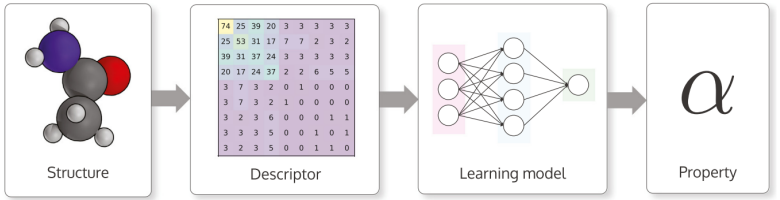
Perhaps one of the most important parts of machine learning is the data. And in this case, another important part is deciding how to interpret such data so that machine learning methods can understand it and use it.

Typically, descriptors are used to interpret chemical data in computers. Think of it as a matrix, where the numbers represent different properties of the chemical structure. DScribe is a Python library offering many different descriptor methods. There is a lot of interesting details about the requirements and properties for ideal descriptor, and there are a couple of different descriptors. We chose a local descriptor method called Smooth Overlap of Atomic Positions (SOAP). (Here I would insert a lot of Math, but I don’t really think it would be very interesting for most people).

Machine Learning Methods

Several existing studies have reviewed and analyzed machine learning algorithms commonly used in chemistry. For our project, we have chosen these models due to their promising results and established applications in similar domains.

Kernel Ridge Regression (KRR) combines Ridge regression and classification (linear least squares with L2-norm regularization) with the kernel trick. It thus learns a linear function in the space induced by the respective kernel and the data.
Gradient Boosting Regression (GBR) produces a predictive model from an ensemble of weak predictive models. Gradient boosting can be used for regression and classification problems.
Neural Networks

The idea was to test these different methods, compare them, and achieve similar results compared to existing relevant research.

Dataset

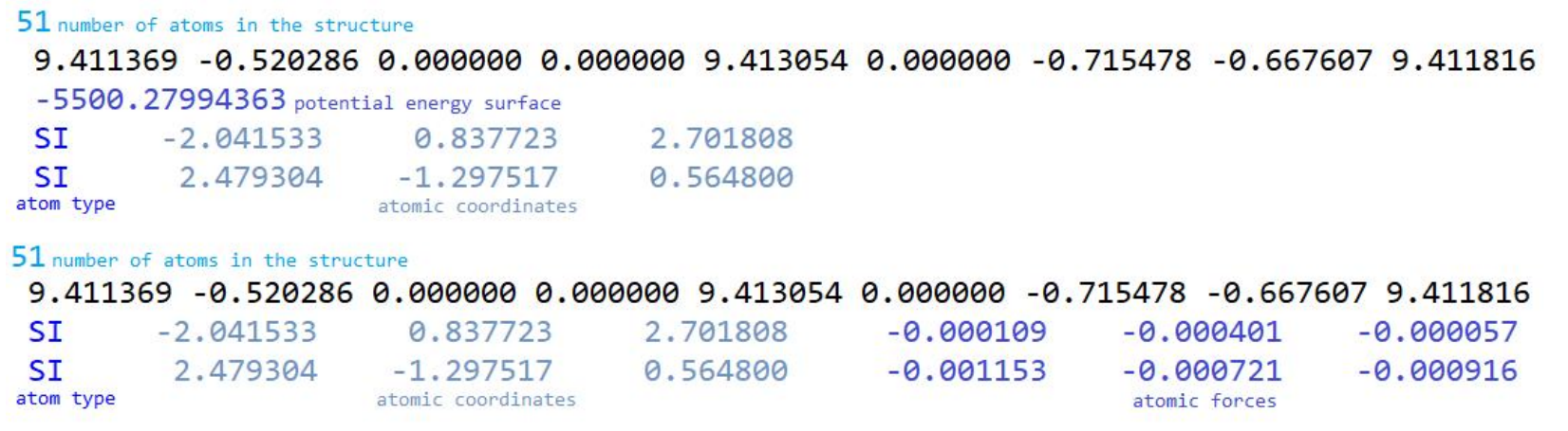
The dataset was provided by Institut Charles Gerhardt Montpellier. It contained 64 084 chemical structures of zeolites with reagents, including energies and atomic forces for four zeolites: CHA (chabazite), FAU (FAU-Y), FER (ferrite) and MOR (mordenite), reacting with mercaptan, methanol, benzene, toluene and phenol. The structures were heated to 673 and 823 K in the reactions. Two reaction mechanisms were taken into account, called stepwise reaction and concerted reaction. The units for the potential energy surface are in a.u. (atomic units), also Hartree (Eh). Units for the atomic forces of the unit in Ry/Bohr. The PES values were calculated using DFT calculations and forces were derived from PES values.

The dataset for atomic forces contains:

number of atoms in each structure
cell parameters xx, xy, xz, yx, yy, yz, zx, zy, zz, name of the structure
atomic coordinates: atom type, x, y, z, atomic forces: x, y, z - values to predict

The dataset for potential energy surface contains:

number of atoms in each structure
cell parameters xx, xy, xz, yx, yy, yz, zx, zy, zz, name of the structure
total energy for each structure - value to predict
atomic coordinates: atom type, x, y, z

After dataset analysis, we identified a small number of outliers. After a discussion with domain experts, we decided to remove 64 structures as outliers. The final number of structures was 64 020.

After converting our raw input data into descriptors, we implemented zero padding to ensure a uniform shape for each structure in the dataset. We divided the dataset into training and testing sets, with an 80:20 ratio. For the neural network model, we split the data into an 80% training set, a 10% validation set, and a 10% testing set. We incorporated an additional dataset comprising 5760 clean zeolites without reagents This dataset included Si, O, one Al, and one H atom per structure. Our objective was to evaluate whether the simplified zeolite structures would yield improved results compared to the full dataset.

def create_soap_descriptor(species):
  cutoff_radius = 10  # Cutoff radius for the SOAP descriptor
  max_radial_order = 3  # Maximum radial basis function order
  max_angular_order = 2  # Maximum angular basis function order

  soap = SOAP(
  species=species,
  # species (iterable) – The chemical species as a list of atomic numbers or as a list of chemical symbols.
  # Notice that this is not the atomic numbers that are present for an individual system,
  # but should contain all the elements that are ever going to be encountered when creating the descriptors for a set of systems.
  # Keeping the number of chemical species as low as possible is preferable.
  periodic=False,  # Set to True if your system is periodic (e.g., crystal structures)
  r_cut=cutoff_radius,
  n_max=max_radial_order, # The number of radial basis functions.
  l_max=max_angular_order, # The maximum degree of spherical harmonics.
  sigma=0.1,   # Width of the Gaussian basis functions (can be adjusted)
  rbf='gto',  # Radial basis function
  #compression={'mode': 'mu2', 'species_weighting': None}
  )

  return soap

Reading the dataset from .txt file, we gather the number of atoms in the structure, then read the cell parameters, total energy (for PES) and then in the range of number of atoms, we read the atom types and their coordinates. At the end, we create a SOAP descriptor. The result is a matrix, where each row represents the local environment of one atom in the molecule.

# start a new structure
num_atoms = int(line)  # get number of atoms in the structure
cell_params = []
line = next(f)  # read next line manually
for i in range(9):  # read 9 cell parameters - xx, xy, xz, yx, yy, yz, zx, zy, zz
    cell_params.append(float(line.split()[i]))
struct_name = line.split()[11]  # read structure name
line = next(f)  # read next time manually
total_energy = float(line)  # read total energy
# read atom types and coordinates until the end of the structure according to the number of atoms
atom_types = []
atom_coords = []
for i in range(num_atoms):
    line = next(f)
    atom_types.append(line.split()[0].capitalize())
    atom_coords.append([float(x) for x in line.split()[1:]])

# create Atoms object
structure = Atoms(symbols=atom_types, positions=atom_coords)
# create SOAP descriptor
soap = create_soap_descriptor(species)
soap_descriptor = soap.create(system=structure)
soap_descriptors.append(soap_descriptor)
# matrix where each row represents the local environment of one atom of the molecule.
# The length of the feature vector depends on the number of species defined in species as well as n_max and l_max
# [number of atoms, number of features for each atom]

Since each structures has different number of atoms, we also added zero-padding to ensure each descriptor has the same shape. The final shape will look as following: (number of structures, max. number of atoms, number of features)

For atomic forces, it was a little more complicated. Each atom in the molecule has three values for forces in each direction (x, y, z). The vector would look like this: (number of structures, max. number of atoms, 3) (3 is the x, y, z forces directions)

We have to also convert these vector from 3D to 2D, as that is the most standard accepted input for machine learning methods.

Thus, the actual final vectors will look like:

SOAP descriptor: (number of structures, max. number of atoms × number of features)
Shape for atomic forces vector: (number of structures, max. number of atoms × 3)

Let’s look at an example: Remember, we have total of 64 020 structures. Let’s imagine that the maximum number of atoms in structures is 151. Thus, for atomic forces, the vector has shape of (64020, 151, 3), and then converted to 2D will result in shape of (64020, 453).

Predictions

We mostly worked with the scikit-learn Python library which provides methods for using KRR and GBR, and additional functions such as grid search. As we discovered at that time, GBR doesn’t support multi-output regression natively, so we ended up not using GBR for predicting the atomic forces. For neural networks, we used TensorFlow library. We experimented with many different types of architectures, activation functions, drop out layers, regularizations, optimizers… (this is the boring part of every experiment. Waiting.)

Additionally, we tested SchNet library for comparison with our methods - see documentation

param_grid = { # hyperparameters to tune
'alpha': [0.001, 0.01, 0.1, 1.0, 10],
'kernel': ['rbf'],
'gamma': [0.001, 0.01, 0.1, 1.0, 10]
}
x_train, x_test, y_train, y_test = train_test_split(soap_descriptors, df_energy['total_energy'].values, test_size=0.2, random_state=0)

### if we enjoy some specific values
krr = KernelRidge(alpha=0.001, kernel='rbf', gamma=1)

### if not, we perform GridSearch
grid_search = GridSearchCV(estimator=krr, param_grid=param_grid, scoring='neg_mean_absolute_error', cv=5)
grid_search.fit(x_train, y_train)
best_estimator = grid_search.best_estimator_
print("Best Hyperparameters:", grid_search.best_params_)

krr.fit(x_train, y_train)
predicted_energy = krr.predict(x_test)
### and then we evaluate the results, we used R2 score, mean squared error, mean absolute error, root mean squared error
r2 = r2_score(y_test, predicted_energy)
.... # and then draw some plots of the predicted energy vs actual energy

GBR was quite similar, but had different hyperparameters, and after figuring out the magic with atomic forces and their shapes, we also performed KRR similarly. Neural network testing was a never-ending story. If you know, you know. Especially with atomic forces. Clearly, predicting three values is not very trivial.

# Pretending I know what I am doing with my life
# This is just one of the examples of neural network architecture, please don't judge me
model = tf.keras.models.Sequential([
    tf.keras.Input(shape=(soap_descriptors.shape[1],)), # num_features
    tf.keras.layers.Masking(mask_value=0.),  # Masking layer to handle padded values
    tf.keras.layers.Dense(16384, activation='linear'),
    tf.keras.layers.BatchNormalization(),
    tf.keras.layers.ReLU(),
    tf.keras.layers.Dropout(0.3),

    tf.keras.layers.Dense(16384, activation='linear'), 
    tf.keras.layers.BatchNormalization(),
    tf.keras.layers.ReLU(),
    tf.keras.layers.Dropout(0.3),

    tf.keras.layers.Dense(atomic_forces_list.shape[1])
])

initial_learning_rate = initial_learning_rate
lr_schedule = tf.keras.optimizers.schedules.ExponentialDecay(
    initial_learning_rate,
    decay_steps=10000,
    decay_rate=0.90,
    staircase=True)
reduce_lr = tf.keras.callbacks.ReduceLROnPlateau(monitor='val_loss', factor=0.1,
                          patience=20, min_lr=1e-7, verbose = 1)
optimizer = tf.keras.optimizers.Adam(learning_rate=0.001)
model.compile(optimizer=optimizer, loss='mean_squared_error', metrics=['mean_squared_error'])
soap_descriptors = soap_descriptors.astype(np.float32)
atomic_forces_list = atomic_forces_list.astype(np.float32)
s_mean = np.mean(soap_descriptors, axis=0, keepdims=True)
s_std = np.std(soap_descriptors, axis=0, keepdims=True)
soap_normalized = (soap_descriptors - s_mean) / (s_std + 0.000001)
scaling_factor = np.longdouble(100000)
# Multiply atomic forces by the scaling factor - I thought this might help, but I don't think it did
atomic_forces_list = atomic_forces_list * scaling_factor
x_train, x_test, y_train, y_test = train_test_split(soap_normalized, atomic_forces_list, test_size=0.1, random_state=42)

Discussing the Results

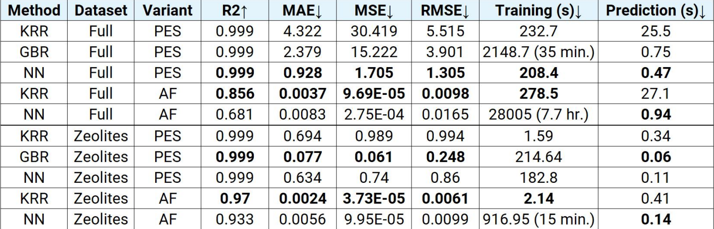
Predicting PES turned out to be pretty simple task. The results were good across all methods with R2 score being 0.999 (R2 of 1.0 is perfect prediction, so 0.999 is essentially ideal), but neural network reached the smallest error, so we considered it as a winner. When it comes to speed however - GBR took the longest to train (35 mins). KRR and NN took around 200 seconds. NN had the fastest prediction time (0.47 seconds!).

Atomic forces were a little more painful. KRR reached R2 score of 0.856, while NN reached 0.681. Here I was hoping for better performance, but while for predicting energy we only predict one value for the whole structure, for AF we are predicting 3 x number of atoms values, which results in bigger output space. NN also took a very long time to train (around 7 hours) compared to KRR (278 seconds).

However, the structures of clear zeolites achieved very good results, which at least served as a proof that I am not doing some nonsense. We did a lot more different experiments - selected only specific type of reactions, descriptor compression, different dataset, different descriptors… to compare all the results.

For SchNet, we chose the PaiNN (polarizable interaction neural network) representation (I see what you did there). In the backend, SchNet uses the PyTorch library. Results for PES were very good (0.999 R2 score and even smaller error than our solution) and for AF the score was similar to what we achieved with our own NN (0.667 R2 Score). However the training took a very long time - 29 hours.

After all of this, I didn’t have enough, and also decided to test if we can predict PES and retrieve AF, since AF are negative derivative of the energy wrt atomic positions.

\[F = −∇E(x, y, z)\]

What this means is: we will iterate over each atom in the structure, move it in each direction (x, y, z) positively and negatively, create a SOAP descriptor, and predict the energy. We then calculate the difference in energy divided by the difference in position. The value δ represents how much we move each atom, need to be chosen carefully. We tested 0.1, 0.001, 0.0001 and 0.00001. To predict the energy, we selected our NN model which achieved the best results. Unfortunately, this didn’t yield very relevant results. Force values are very sensitive to change, or energy, and therefore an even more accurate model would probably be needed to achieve better results. But it was interesting!

# create the soap descriptor - move the atomic coordinates by delta in both directions
def process_dataset(file_name, species, model, delta):
  soap_descriptors = []
  energy_list = []
  atomic_forces_list_predictions = []
  max_num_atoms = 151
  with open(file_name, 'r') as f:
      for line in f:
          if line.strip().isdigit():
              # start a new structure
              num_atoms = int(line)  # get number of atoms in the structure
              cell_params = []
              line = next(f)  # read next line manually
              for i in range(9):  # read 9 cell parameters - xx, xy, xz, yx, yy, yz, zx, zy, zz
                  cell_params.append(float(line.split()[i]))
              struct_name = line.split()[11]  # read structure name
              print(struct_name)
              line = next(f)  # read next time manually
              total_energy = float(line)  # read total energy
              # read atom types and coordinates until the end of the structure according to the number of atoms
              atom_types = []
              atom_coords = []
              for i in range(num_atoms):
                  line = next(f)
                  atom_types.append(line.split()[0].capitalize())
                  atom_coords.append([float(x) for x in line.split()[1:]])
              for i in range(num_atoms):
                  for dim in range(3):

                      # Moving in both directions by delta
                      new_atom_coords_plus  = [coord[:] for coord in atom_coords]
                      new_atom_coords_plus[i][dim] += delta

                      new_atom_coords_minus = [coord[:] for coord in atom_coords]
                      new_atom_coords_minus[i][dim] -= delta

                      structure_plus = Atoms(symbols=atom_types, positions=new_atom_coords_plus)
                      structure_minus = Atoms(symbols=atom_types, positions=new_atom_coords_minus)
                      structure = Atoms(symbols=atom_types, positions=atom_coords)

                      # create SOAP descriptor
                      soap_plus = create_soap_descriptor(species)
                      soap_descriptor_plus = soap_plus.create(system=structure_plus)

                      soap_minus = create_soap_descriptor(species)
                      soap_descriptor_minus = soap_minus.create(system=structure_minus)

                      # Padding
                      num_atoms = soap_descriptor_plus.shape[0] # reusing the variable for padding logic
                      if num_atoms < max_num_atoms:
                          soap_descriptor_plus = np.pad(soap_descriptor_plus,((0, max_num_atoms - num_atoms), (0, 0)), 'constant',constant_values=0)
                          soap_descriptor_minus = np.pad(soap_descriptor_minus,((0, max_num_atoms - num_atoms), (0, 0)), 'constant',constant_values=0)

                      soap_descriptor_plus = soap_descriptor_plus.reshape(1, -1)

                      soap_descriptor_minus = soap_descriptor_minus.reshape(1, -1)

                      # Normalization needed for NN model
                      s_mean = np.loadtxt('dataset/s_mean.txt')
                      s_std = np.loadtxt('dataset/s_std.txt')

                      soap_descriptor_plus = soap_descriptor_plus.astype(np.float32)
                      soap_descriptor_plus_normalized = (soap_descriptor_plus - s_mean) / (s_std + 0.000001)

                      soap_descriptor_minus = soap_descriptor_minus.astype(np.float32)
                      soap_descriptor_minus_normalized = (soap_descriptor_minus - s_mean) / (s_std + 0.000001)

                      # Predicting for each direction
                      predicted_energy_plus = model.predict(soap_descriptor_plus_normalized)
                      predicted_energy_minus = model.predict(soap_descriptor_minus_normalized)
                      # Calculate the final Force component -> in total 3 x number of atoms
                      force_component = (predicted_energy_plus - predicted_energy_minus) / (2 * delta)
                      atomic_forces_list_predictions.append(force_component)

Conclusion

Our solution has the potential to help specialists and domain experts speed up chemical calculations. A limitation of our solution was the insufficient accuracy of atomic force prediction for zeolites. Improvements could include expanding the dataset, more extensive training, or an even better potential energy surface model to derive atomic forces. However, even in comparison with the SchNet solution, it can be said that force prediction is more complicated, and the complexity stems from the nature of this chemical property. The use of other descriptors to describe the chemical environment also showed good potential. Other properties may also depend on the type of zeolite or the type of reaction mechanism, as we observed in our experiments.

My personal conclusion would be probably that this was a lot of work. I felt like the only person who understood this in the whole country was my thesis supervisor. It ended up being difficult to defend this thesis as you can imagine. We actually had two defences. The first one gave me PTSD. The second one - I was the first person to become an engineer as they call people with Master’s degree. (Monday, 8am, thesis defended, went home, but joked about just going straight to work). The biggest challenge was probably the fight with myself and believing that I can actually do this. I had a lot of moments when the results weren’t good, the predictions were off, and I thought that it just won’t work. Even with good results, I kept feeling that I must be doing something wrong, these results are too good to be true. But in the end, I am very proud of myself for tackling this challenge and graduating (with an A, yay!). (But I would not do it again 😂).